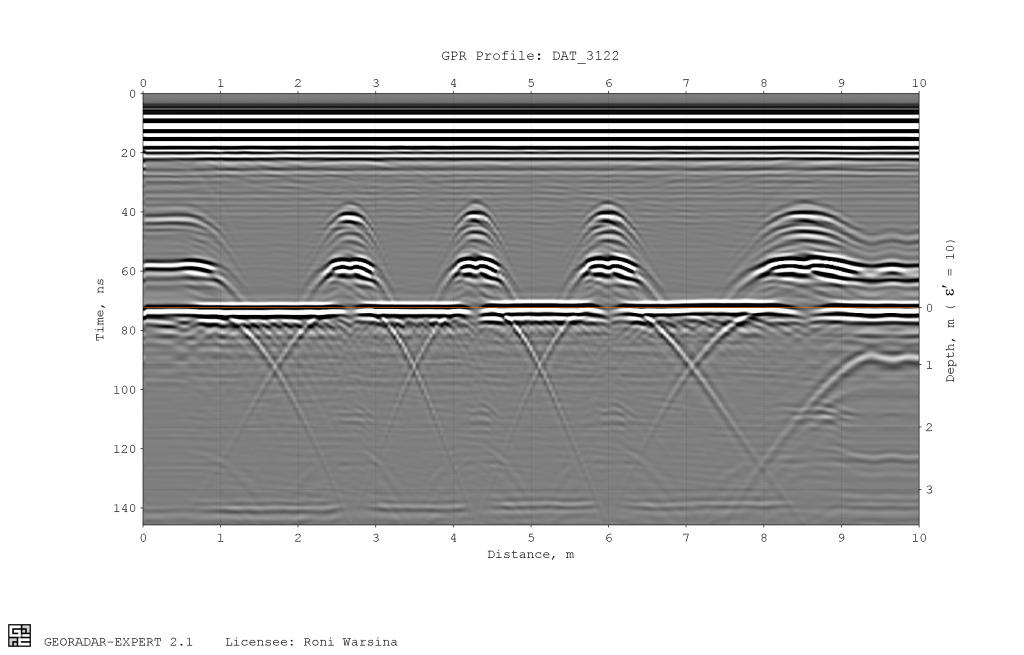
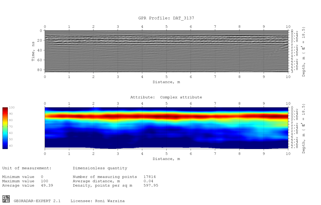
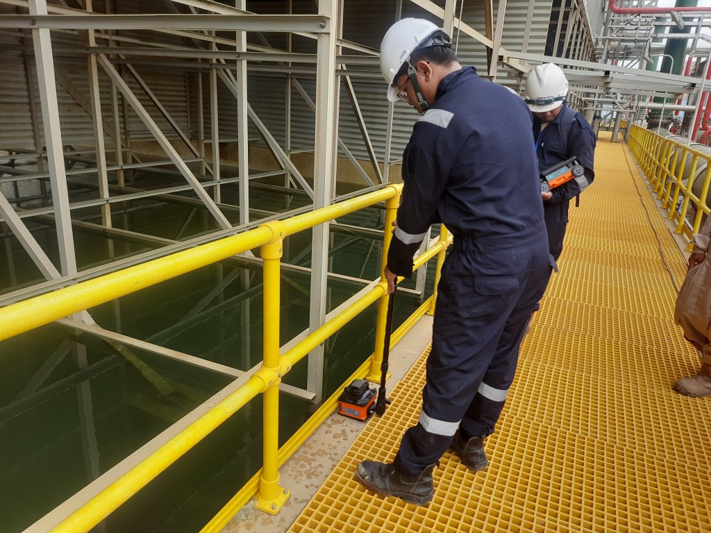
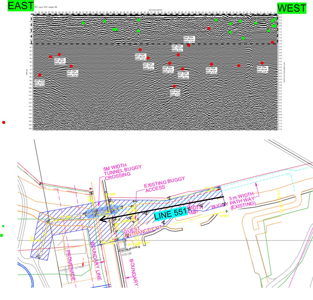
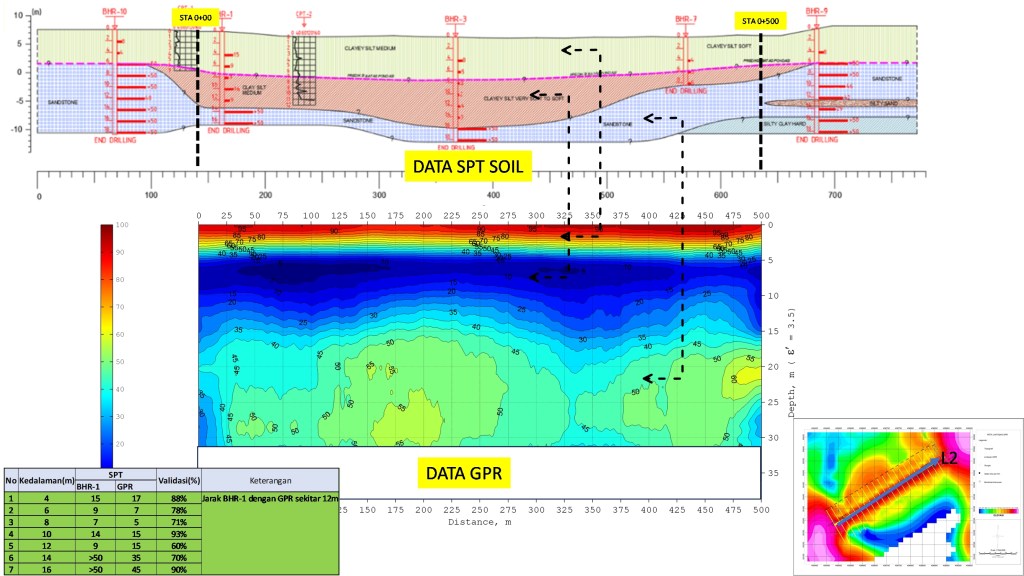
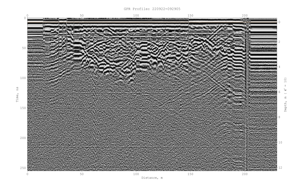
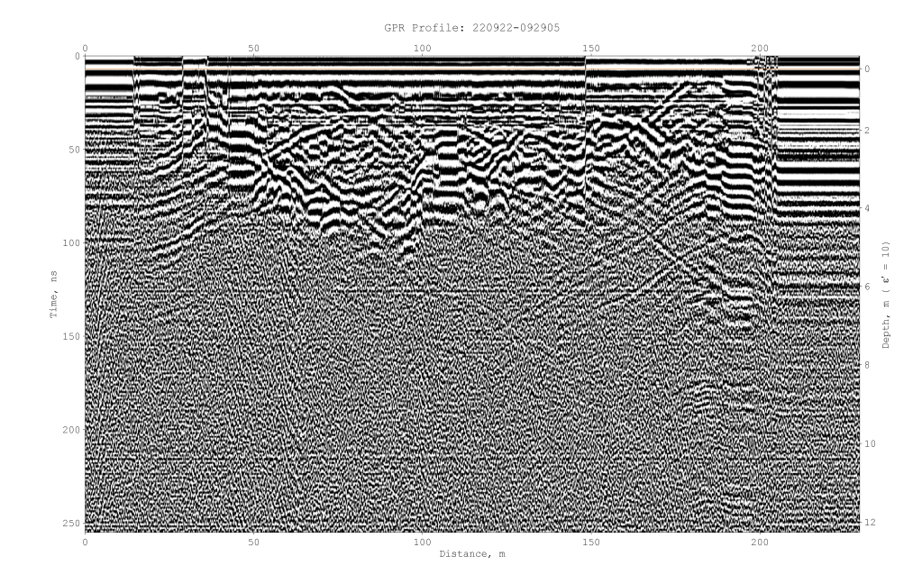
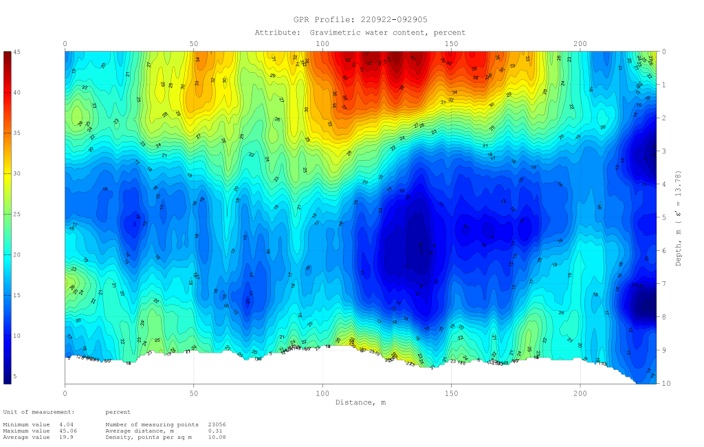
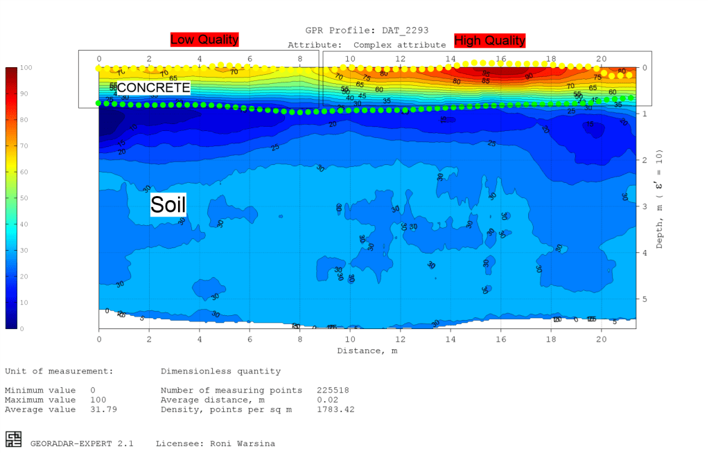
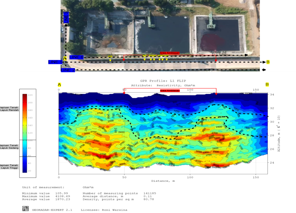
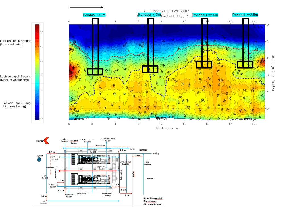
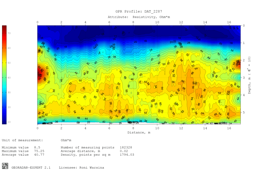
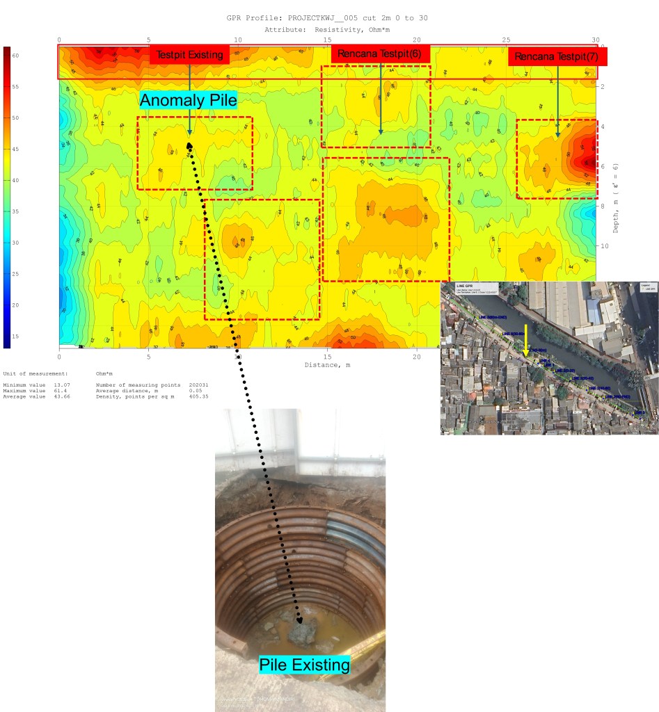
Seisxplore Survey
Konsultan Geofisika|Geologi|Geoteknik
-

-

The microgravity survey using Scintrex CG-5 and CG-6 involves precise measurements of small variations in the Earth’s gravitational field. These variations can help detect subsurface density anomalies, which are useful in geotechnical, hydrogeological, and exploration applications. Below are key aspects of conducting a microgravity survey with these instruments.
1. Introduction to Scintrex CG-5 & CG-6
Scintrex CG-5 and CG-6 are high-precision relative gravimeters designed for microgravity surveys. The CG-6 is an updated version of the CG-5, featuring improved electronics, better thermal stability, and enhanced data acquisition capabilities.
Key Features
Feature Scintrex CG-5 Scintrex CG-6 Accuracy ±1 µGal ±0.8 µGal Resolution 0.1 µGal 0.01 µGal Drift Rate <10 µGal/day <5 µGal/day Display LCD Screen Touchscreen Data Storage Internal + External Larger internal storage Battery Life ~24 hours ~30 hours
2. Microgravity Survey Workflow
Step 1: Survey Planning
- Define the objective (e.g., cavity detection, groundwater studies, fault mapping).
- Select survey grid and station spacing (typically 5–50 meters depending on target resolution).
- Identify and record base station locations for drift correction.
Step 2: Instrument Setup
- Place the gravimeter on a stable tripod.
- Level the instrument using the bubble level and adjustable legs.
- Allow the instrument to stabilize before taking measurements.
- Input station coordinates (manually or via GPS if supported).
Step 3: Data Acquisition
- Take multiple readings at each station to minimize noise.
- Record environmental conditions (temperature, pressure) to aid in corrections.
- Measure at a base station periodically to track instrument drift.
Step 4: Data Processing & Corrections
Apply standard gravity corrections:
- Drift Correction – Remove instrument drift by referencing base station readings.
- Tidal Correction – Account for Earth and lunar tidal effects.
- Latitude Correction – Adjust for gravity variations with latitude.
- Free-Air Correction – Correct for elevation differences.
- Bouguer Correction – Remove gravitational effect of overburden.
- Terrain Correction – Adjust for local topographic variations.
Step 5: Interpretation
- Generate Bouguer anomaly maps.
- Identify density variations indicating subsurface structures.
- Correlate results with geological, geotechnical, or hydrogeological data.
3. Advantages of CG-5 & CG-6 in Microgravity Surveys
- High sensitivity to small density variations.
- Robust design for fieldwork with minimal maintenance.
- CG-6 offers enhanced automation and data storage.


-

The resistivity method is an effective geophysical technique for detecting subsurface cavities. The SuperSting R8 is an advanced multi-channel resistivity imaging system used to map electrical resistivity variations in the subsurface, which helps identify voids, sinkholes, or other anomalies.
1. Principles of Cavity Detection Using Resistivity
Cavities, voids, and air-filled spaces exhibit high resistivity because air (or dry voids) is a poor conductor of electricity. Conversely, water-filled cavities can have either moderate or low resistivity, depending on the water’s salinity.
Resistivity Trends for Different Subsurface Materials
Material Resistivity Range (Ωm) Air-filled cavity Very high (>1000 Ωm) Water-filled cavity Moderate (10–100 Ωm) Clayey soil Low (1–50 Ωm) Sandy soil Moderate (50–500 Ωm) Limestone (intact) Moderate (100–1000 Ωm)
2. Data Acquisition with SuperSting R8
Survey Design
- Choose electrode spacing based on the expected cavity size and depth (e.g., 1–5 meters spacing).
- Use a 2D or 3D resistivity survey for a comprehensive image.
- Common array types:
- Dipole-Dipole (good for lateral resolution and deeper cavities).
- Wenner-Schlumberger (balanced sensitivity for depth and lateral variations).
- Gradient Array (fast for large-area surveys).
Field Procedure
- Set up the electrode line with stainless steel or graphite electrodes.
- Connect electrodes to the SuperSting R8 system using the switch box.
- Select survey parameters (e.g., current injection, stacking, measurement cycles).
- Start data acquisition, allowing SuperSting R8 to record resistivity values at multiple depths.
3. Data Processing & Interpretation
Step 1: Data Filtering
- Remove noisy or outlier readings caused by poor electrode contact or interference.
- Apply topographic corrections if necessary.
Step 2: Resistivity Inversion
- Use software like EarthImager 2D/3D or Res2DInv to convert raw apparent resistivity into a depth model.
- Generate a pseudosection and a true resistivity model.
Step 3: Identifying Cavities
- Look for high-resistivity anomalies (possible air-filled cavities).
- Water-filled cavities appear as moderate resistivity zones.
- Ensure anomalies are not due to boulders, compacted zones, or artifacts.
Example Interpretation
- High-resistivity (≥1000 Ωm) = Possible air-filled void.
- Moderate resistivity (50–500 Ωm) = Water-filled void.
- Surrounding low to moderate resistivity = Normal soil or weathered rock.
4. Case Study Example
Survey Setup:
- Electrode spacing: 2m
- Array used: Dipole-Dipole
- Depth of investigation: 10–15m
Results:
- A high-resistivity anomaly (~1500 Ωm) at 5m depth, 4m wide, suggesting an air-filled cavity.
- A moderate-resistivity anomaly (~100 Ωm) at 10m depth, possibly indicating a water-filled void.
5. Advantages of Using SuperSting R8 for Cavity Detection
✔ Multi-channel system → Faster data acquisition.
✔ High-resolution imaging → Clearer subsurface details.
✔ Compatible with 2D and 3D surveys → Better spatial coverage.
✔ Supports multiple array types → More flexibility for different site conditions.


-

Limestone formations are highly susceptible to karstification, leading to the formation of voids, sinkholes, and cavities. The resistivity method is one of the most effective geophysical techniques for detecting these subsurface anomalies.
This guide outlines the best practices for conducting a resistivity survey for cavity detection in limestone using SuperSting R8.
1. Why Use Resistivity for Cavity Detection?
Cavities have distinct electrical properties compared to the surrounding limestone.
- Air-filled cavities → Very high resistivity (>1000 Ωm)
- Water-filled cavities → Moderate resistivity (10–500 Ωm, depending on water salinity)
- Intact limestone → 100–1000 Ωm
- Weathered limestone/clay infill → Low resistivity (1–50 Ωm)
2. Survey Design and Field Setup
Survey Planning
- Define the survey area based on geological and structural conditions.
- Choose an appropriate electrode spacing (typically 2–5 meters for near-surface cavities).
- Determine the depth of investigation (1/3 to 1/5 of the survey line length).
Electrode Array Selection
Array Type Advantages Recommended Use Dipole-Dipole High lateral resolution, good for detecting cavities Best for mapping horizontal and vertical voids Wenner-Schlumberger Balanced depth and lateral resolution Useful when both depth and shape of voids are unknown Gradient Rapid data collection, good for large areas Suitable for large-scale reconnaissance surveys Pole-Dipole Good depth penetration Used when deep cavities are suspected
Field Setup Using SuperSting R8
- Lay out the electrode line over the survey area.
- Insert electrodes into the ground at regular intervals.
- Connect electrodes to the SuperSting R8 using a switch box.
- Configure survey parameters:
- Select array type (e.g., Dipole-Dipole for cavities).
- Set current injection and stacking to reduce noise.
- Start data acquisition and monitor real-time data for anomalies.
3. Data Processing & Interpretation
Step 1: Data Pre-Processing
- Remove noisy readings from poor electrode contact.
- Apply topographic corrections if needed.
Step 2: Resistivity Inversion
Use software like EarthImager 2D/3D or Res2DInv to generate a resistivity model.
- Air-filled cavities appear as very high resistivity anomalies (>1000 Ωm).
- Water-filled cavities show moderate resistivity (10–500 Ωm).
- Clay-filled voids appear as low-resistivity zones (1–50 Ωm).
- Weathered limestone has a more gradual resistivity variation.
Step 3: Identifying Cavity Anomalies
- Look for high-resistivity zones that contrast sharply with surrounding limestone.
- Verify anomaly shape: irregular, rounded, or vertically elongated structures suggest karst cavities.
- Cross-check with borehole or GPR data (if available) for confirmation.
4. Case Study Example
Survey Setup
- Electrode spacing: 3m
- Array type: Dipole-Dipole
- Survey length: 60m
- Depth of investigation: ~15m
Results
- A high-resistivity anomaly (~2000 Ωm) at 6m depth, approximately 5m wide → Indicates a possible air-filled cavity.
- A moderate-resistivity zone (~100 Ωm) at 12m depth → Possible water-filled void.
- Low-resistivity region (~30 Ωm) surrounding the void → Suggests clay or weathered limestone infill.
5. Conclusion & Recommendations
✔ Use Dipole-Dipole for high-resolution cavity mapping.
✔ Combine resistivity with borehole/GPR data for verification.
✔ Perform repeat surveys if seasonal groundwater changes are expected.


-
Geolistrik adalah metode yang sangat efektif untuk eksplorasi air tanah dan akuifer, terutama di daerah perkebunan sawit yang didominasi oleh sedimen pasir. Metode ini membantu mengidentifikasi kedalaman, ketebalan, dan kualitas air tanah, serta membedakan lapisan yang mengandung air dari yang tidak.
1. Prinsip Geolistrik dalam Eksplorasi Air Tanah
Air tanah mempengaruhi nilai resistivitas listrik. Umumnya:
- Lapisan jenuh air → Resistivitas rendah (1–50 Ωm)
- Pasir kering → Resistivitas sedang (50–500 Ωm)
- Pasir jenuh air → Resistivitas rendah (5–50 Ωm, tergantung mineralisasi air)
- Lempung/Clay → Resistivitas sangat rendah (1–10 Ωm, tidak permeabel)
Di kebun sawit yang dominan sedimen pasir, akuifer sering berada di lapisan pasir jenuh air dengan resistivitas rendah hingga sedang.
2. Pemilihan Metode dan Desain Survey
Untuk eksplorasi air tanah di perkebunan sawit, metode Vertical Electrical Sounding (VES) atau 2D Resistivity Imaging sangat direkomendasikan.
Pemilihan Konfigurasi Elektroda
Konfigurasi Kelebihan Kekurangan Schlumberger Baik untuk eksplorasi air tanah yang dalam Waktu pengukuran lebih lama Wenner-Schlumberger Kombinasi kedalaman dan resolusi lateral yang baik Butuh banyak titik pengukuran Dipole-Dipole Resolusi lateral tinggi, cocok untuk akuifer dangkal Kedalaman terbatas Desain Survey
- Jarak antar elektroda: 5–10 meter untuk eksplorasi dangkal, 10–20 meter untuk eksplorasi dalam.
- Panjang lintasan: 200–400 meter untuk mendapatkan gambaran luas.
- Jumlah titik pengukuran: Semakin banyak titik, semakin detail hasil interpretasi.
3. Pengambilan Data di Lapangan
Langkah-langkah Pengukuran
- Persiapan Lokasi
- Identifikasi daerah dengan potensi air tanah tinggi (cek topografi, vegetasi, dan sumur terdekat).
- Pastikan tanah tidak terlalu kering atau terlalu basah untuk kontak elektroda yang baik.
- Pemasangan Elektroda
- Gunakan elektroda stainless steel atau grafit.
- Jarak elektroda disesuaikan dengan target kedalaman.
- Pengambilan Data dengan SuperSting R8
- Hubungkan elektroda ke alat geolistrik SuperSting R8.
- Pilih metode pengukuran (Schlumberger atau Wenner-Schlumberger).
- Atur parameter arus dan tegangan untuk mendapatkan sinyal optimal.
- Pengecekan Kualitas Data
- Lakukan stacking (pengulangan pengukuran) untuk mengurangi noise.
- Pastikan nilai resistivitas tidak menunjukkan anomali akibat gangguan eksternal.
4. Interpretasi Data dan Identifikasi Akuifer
Tahapan Analisis
- Filtering Data
- Hapus anomali akibat kontak elektroda yang buruk atau gangguan eksternal.
- Koreksi topografi jika ada perubahan elevasi signifikan.
- Inversi Data
- Gunakan software Res2DInv atau EarthImager 2D untuk mendapatkan profil resistivitas bawah permukaan.
- Identifikasi zona resistivitas rendah (5–50 Ωm) yang menunjukkan keberadaan akuifer.
- Interpretasi Akuifer
- Pasir jenuh air → Resistivitas 5–50 Ωm, indikasi akuifer potensial.
- Lapisan lempung → Resistivitas <10 Ωm, bisa menjadi pembatas akuifer.
- Pasir kering atau batuan keras → Resistivitas >100 Ωm, bukan akuifer.
Contoh Hasil
- Akuifer ditemukan pada kedalaman 10–25 meter dengan ketebalan sekitar 15 meter.
- Air berpotensi tersedia dalam jumlah besar jika formasi pasir cukup tebal.
- Jika terdapat lapisan lempung di atas akuifer, kemungkinan akuifer tertekan (confined).
5. Kesimpulan dan Rekomendasi
✔ Gunakan metode Schlumberger atau Wenner-Schlumberger untuk eksplorasi air tanah di sedimen pasir.
✔ Lapisan pasir jenuh air (5–50 Ωm) menunjukkan zona akuifer potensial.
✔ Hindari lapisan lempung sebagai sumber air karena permeabilitasnya rendah.
✔ Gunakan sumur uji untuk verifikasi hasil geolistrik sebelum pengeboran sumur produksi.


-
Dalam eksplorasi air tanah menggunakan survey geolistrik, langkah utama adalah menentukan volume akuifer dan memperkirakan cadangan air tanah berdasarkan hasil resistivitas.
1. Identifikasi Akuifer dari Hasil Geolistrik
Setelah melakukan survey geolistrik menggunakan Schlumberger atau Wenner-Schlumberger, akuifer dapat diidentifikasi berdasarkan resistivitas:
- Pasir jenuh air → 5–50 Ωm (akuifer potensial)
- Lempung → <10 Ωm (bukan akuifer)
- Batuan keras → >100 Ωm (non-akuifer)
Dari hasil interpretasi geolistrik, tentukan parameter berikut:
- Ketebalan akuifer (h) dalam meter
- Luas area akuifer (A) dalam meter persegi
- Porositas efektif (n) dalam persen
- Koefisien penyimpanan (S) untuk air tanah dalam atau akuifer tertekan
2. Perhitungan Cadangan Air Tanah
Cadangan air tanah dapat dihitung menggunakan rumus:
1. Volume Air Tersedia dalam Akuifer
V=A×h×nV = A \times h \times n
Dimana:
- VV = Volume air yang dapat disimpan (m³)
- AA = Luas area akuifer (m²)
- hh = Ketebalan akuifer (m)
- nn = Porositas efektif (% → dalam desimal)
2. Debit Air yang Bisa Diambil (Q)
Jika ingin mengetahui debit air yang bisa diambil dari akuifer: Q=S×A×hQ = S \times A \times h
Dimana:
- QQ = Debit maksimum (m³/hari)
- SS = Koefisien penyimpanan (untuk akuifer bebas: 0.01–0.30, akuifer tertekan: 0.0001–0.01)
Contoh Perhitungan:
Dari hasil survey geolistrik:- Luas akuifer (A) = 5000 m²
- Ketebalan akuifer (h) = 20 m
- Porositas efektif (n) = 0.25 (25%)
Maka, volume air tersedia: V=5000×20×0.25=25,000 m³V = 5000 \times 20 \times 0.25 = 25,000 \text{ m³}
Jika koefisien penyimpanan (S = 0.02 untuk akuifer bebas), maka debit air per hari: Q=0.02×5000×20=2000 m³/hariQ = 0.02 \times 5000 \times 20 = 2000 \text{ m³/hari}
3. Rekomendasi Titik Bor Air Tanah
Kriteria Pemilihan Lokasi Sumur Bor
✔ Dekat dengan anomali resistivitas rendah (menunjukkan air tanah jenuh)
✔ Hindari zona resistivitas sangat rendah (<5 Ωm) → bisa jadi lempung (impermeabel)
✔ Cek kedalaman akuifer optimal (hasil geolistrik menunjukkan ketebalan 10–30 m)
✔ Jauh dari polusi atau sumber kontaminasi (misal septic tank, limbah)
✔ Dekat dengan area kebutuhan air (agar efisien dalam distribusi)Metode Verifikasi Titik Bor
- Survey tambahan (GPR atau borehole logging) untuk konfirmasi zona jenuh air
- Pengeboran sumur uji (piezometer) untuk mengukur kedalaman air tanah
- Uji debit air untuk memastikan akuifer cukup produktif
4. Kesimpulan & Rekomendasi
✔ Gunakan hasil geolistrik untuk menentukan ketebalan dan luas akuifer
✔ Hitung volume air berdasarkan luas area dan porositas
✔ Pilih titik bor di zona resistivitas 5–50 Ωm yang menunjukkan pasir jenuh air
✔ Lakukan uji debit sebelum menentukan sumur produksidi bawah adalah perhitungan volume air dari nilai resistivitas yang sudah dilakukan di lapangan dengan menggunakan software pendukung. Volume tersebut masih berupa air dan materialnya sehingga perlu dilakukan persentase kandungan air dari total volume yang dihitung.


